Our discussion of public goods seemed incomplete without at least a little math to back it up. But no one wants to alienate the mathophobes, so we parked this tidbit in the “appendix.”
Let’s analyze a few public goods. Imagine, again, 5 farmers. Last year, one farmer contracted with a beekeeper to manage a hive of bees near his field. He paid $2500 for the year. The next year, his harvest increased by $4500. A farmer in a nearby neighborhood paid for even more hives and boosted his profits even more, although the first $2500 is the most effective in this regard.
But he’s not the only one who benefits. Each of this neighbors also increased their crop yields. After doing some research, he discovers that, in a community such as theirs, for each of your neighbors hiring a $2500 bee hive, you can get $1500 more crop even without spending a cent on your own bees. Mathematically, let’s conjecture that the value of the increased yield is
[latex]\sqrt{\alpha S_0 + \sum \beta S_i}[/latex]
and the profit from that extra spending is
[latex]\mbox{Profit}= \sqrt{\alpha S_0 + \sum \beta S_i} – S_0[/latex]
where $latex S_0$ is the amount I spend on bees and $latex S_i$ are my neighbors’ spending. The constant (exogenous) parameters $latex \alpha$ and $latex \beta$ control just how much benefit I get from my own and from my neighbors’ spending, respectively. The reason for the square root is the idea of “diminishing marginal utility.” Spending $6000 on bees is still better than spending $3000, but something less than twice as good. Your first dollar is more important than any subsequent dollar. That said, the utility curve does not have to be a square root.
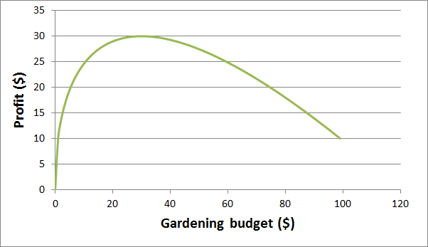
Now, if all of the neighbors are equally interested in their property values, they might agree to all spend the same on bees, perhaps in a written agreement. If we constrain all of $latex S_i$ to be the same value, we have a formula of just one variable and can plot the profit function:
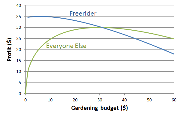
From the plot, we can see that, if the neighbors all cooperate, they can each get $6000 more crop from spending just $3000 on bees. This is the most efficient level of spending. But here we run into the free rider problem. Suppose the neighbors do not cooperate and one of the neighbors does the calculation without considering anyone else. If everyone else continues spending $3000, how much should I spend to maximize my profit? When we fix $latex S_i$ at $3000 and allow just $latex S_0$ to vary, the new plot looks like this:
The neighbors cooperating can make a $3000 profit, but from the blue curve we see that the selfish neighbor can spend just $500 on bees and make a $3500 profit. In this situation, the self-interest of the individual hinders the prosperity of the community.
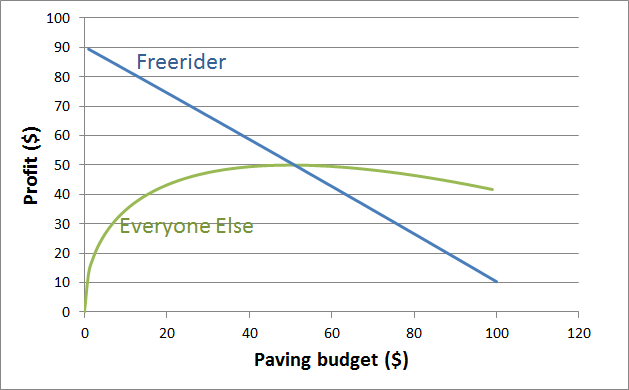
The situation gets even worse for goods which are more public. Perhaps the road leading between the town and the farms needs fixing and they’re freestaters, so the government won’t do it. They’re on their own. This fix will reduce wear on the trucks that take crops to the markets, etc.. Mathematically, $latex \alpha = \beta$. In that case the plot looks like this:
A free-rider, in this case, would have almost no incentive to contribute. That’s not exactly true since even the free riders understand they’re gaming the system and that others will be inclined to seek the same deal. When you incorporate this, you find that, in fact, neighbors are willing to spend just $200 on paving, leaving $3200 of profit on the table. (For more details on this aspect, check out the appendix to the appendix, Galt-ifying Public Goods.) The problem only gets worse as the community grows. If you’re paving a street that benefits 20 people with the same utility function, people are willing to contribute just $47 and will miss out on more than $20,000 profit.
Public goods are not always so easily quantified and it’s usually there that disagreements arise, but a little math goes a long way toward appreciating that opinions about public spending are a continuum and that pretending the market is always right (or always wrong) has real consequences.
Not enough math yet? Check out the appendix to the appendix, where we ask the mathematical question, how much more efficient would John Galt’s community (from the novel Atlas Shrugged) have to be to make up for refusing to subsidize public goods.


