Appendix – This Week In Stupid

Our discussion of public goods seemed incomplete without at least a little math to back it up. But no one wants to alienate the mathophobes, so we parked this tidbit in the “appendix.”

Let’s analyze a few public goods. Imagine, again, 5 farmers. Last year, one farmer contracted with a beekeeper to manage a hive of bees near his field. He paid $2500 for the year. The next year, his harvest increased by $4500. A farmer in a nearby neighborhood paid for even more hives and boosted his profits even more, although the first $2500 is the most effective in this regard.

But he’s not the only one who benefits. Each of this neighbors also increased their crop yields. After doing some research, he discovers that, in a community such as theirs, for each of your neighbors hiring a $2500 bee hive, you can get $1500 more crop even without spending a cent on your own bees. Mathematically, let’s conjecture that the value of the increased yield is

[latex]\sqrt{\alpha S_0 + \sum \beta S_i}[/latex]

and the profit from that extra spending is

[latex]\mbox{Profit}= \sqrt{\alpha S_0 + \sum \beta S_i} – S_0[/latex]

where $latex S_0$ is the amount I spend on bees and $latex S_i$ are my neighbors’ spending. The constant (exogenous) parameters $latex \alpha$ and $latex \beta$ control just how much benefit I get from my own and from my neighbors’ spending, respectively. The reason for the square root is the idea of “diminishing marginal utility.” Spending $6000 on bees is still better than spending $3000, but something less than twice as good. Your first dollar is more important than any subsequent dollar. That said, the utility curve does not have to be a square root.

Now, if all of the neighbors are equally interested in their property values, they might agree to all spend the same on bees, perhaps in a written agreement. If we constrain all of $latex S_i$ to be the same value, we have a formula of just one variable and can plot the profit function:

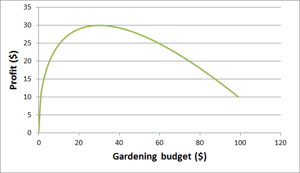
From the plot, we can see that, if the neighbors all cooperate, they can each get $6000 more crop from spending just $3000 on bees. This is the most efficient level of spending. But here we run into the free rider problem. Suppose the neighbors do not cooperate and one of the neighbors does the calculation without considering anyone else. If everyone else continues spending $3000, how much should I spend to maximize my profit? When we fix $latex S_i$ at $3000 and allow just $latex S_0$ to vary, the new plot looks like this:

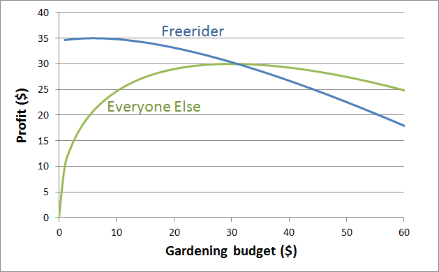
The neighbors cooperating can make a $3000 profit, but from the blue curve we see that the selfish neighbor can spend just $500 on bees and make a $3500 profit. In this situation, the self-interest of the individual hinders the prosperity of the community.

The situation gets even worse for goods which are more public. Perhaps the road leading between the town and the farms needs fixing and they’re freestaters, so the government won’t do it. They’re on their own. This fix will reduce wear on the trucks that take crops to the markets, etc.. Mathematically, $latex \alpha = \beta$. In that case the plot looks like this:

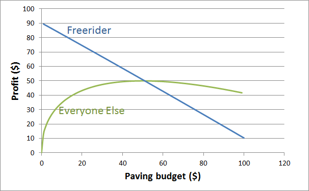
A free-rider, in this case, would have almost no incentive to contribute. That’s not exactly true since even the free riders understand they’re gaming the system and that others will be inclined to seek the same deal. When you incorporate this, you find that, in fact, neighbors are willing to spend just $200 on paving, leaving $3200 of profit on the table. (For more details on this aspect, check out the appendix to the appendix, Galt-ifying Public Goods.) The problem only gets worse as the community grows. If you’re paving a street that benefits 20 people with the same utility function, people are willing to contribute just $47 and will miss out on more than $20,000 profit.

Public goods are not always so easily quantified and it’s usually there that disagreements arise, but a little math goes a long way toward appreciating that opinions about public spending are a continuum and that pretending the market is always right (or always wrong) has real consequences.

Not enough math yet? Check out the appendix to the appendix, where we ask the mathematical question, how much more efficient would John Galt’s community (from the novel Atlas Shrugged) have to be to make up for refusing to subsidize public goods.

See how deep the rabbit hole goes…

In our first appendix, we wandered a little into the math behind public goods. That post has less algebra and more graphs. If what you read here is moving too fast, that might be a good place to start.

Public goods, in brief, are goods which you don’t have to own to enjoy. These are things like public parks, an army, or your neighbor’s front lawn. In that post, we assumed a particular form for a utility function for public goods.

[latex] \mbox{Utility} = \sqrt{\alpha S_0 + \sum\beta S_i}[/latex]

where $latex S_0$ is the amount I spend on the good, $latex S_i$ are my neighbors’ spending. The parameters, $latex \alpha$ and $latex \beta$ determine how much benefit I get from my own spending and my neighbors’ spending, respectively. There’s more on why this specific functional form was chosen here. Other forms are certainly valid.

In this model, the profit is the utility minus my expenditure, $latex S_0$

[latex] \mbox{Profit} = \sqrt{\alpha S_0 + \sum\beta S_i} – S_0[/latex].

If an overbearing government (or home owners association, or business) enforced the same spending on public goods by all beneficiaries, we can determine the optimal spending by equating $latex S_0$ and $latex S_i$ and taking the derivative of profit with respect to this single variable:

[latex] \frac{dP}{dS} = \frac{\alpha+(n-1)\beta}{2\sqrt{S(\alpha+(n-1)\beta)}} – 1[/latex]

Here we’ve introduced n, the total number of participants. Equating this derivative to zero, we find that the optimum level of spending is

[latex] S = \frac{\alpha + (n-1)\beta}{4} [/latex]

for a profit of

[latex] P = \frac{\alpha+(n-1)\beta}{4} [/latex].

per person.

If, on the other hand, we leave it up to each individual to contribute what she thinks is best for herself, we differentiate the profit equation with respect to changes in $latex S_0$ alone.

[latex] \frac{\partial P}{\partial S_0} = \frac{\alpha}{2\sqrt{\alpha S_0+\beta \sum S_i}} – 1[/latex]

Then, since all the participants are assumed to be 100% rational (and will therefore make the same decision), we equate $latex S_0$ and $latex S_i$, set the derivative equal to zero and discover that spending becomes

[latex] \frac{\alpha^2}{4(\alpha + (n-1)\beta)}[/latex]

and profit is

[latex] \frac{\alpha}{2}-\frac{\alpha^2}{4(\alpha+(n-1)\beta)}[/latex].

In the other post on public goods,we reported that, for our simple model of paving the street leading to a cul-de-sac with 5 houses, our homeowners would only be willing, on their own, to spend $2 on paving rather than the ideal $50, which reduced their profit from $50 to $18 each.

Now, let’s introduce a “Galt factor,” G, representing the increased productivity of workers in John Galt’s mountain enclave due to the absence of moochers. How high would the Galt factor have to be for the Galt society to have more efficient lawn care than us regular shmoes? Both $latex S_0$ and $latex S_i$ should be multiplied by G since the labor and other input in the Galt society is that much more potent. So, we multiply all $latex S_0$ and $latex S_i$ by G in the profit for the non-cooperative profit and equate that to the (unmodified) profit for the cooperative system.

[latex] \frac{G\alpha}{2} – \frac{G\alpha^2}{4(\alpha+(n-1)\beta)} = \frac{\alpha+(n-1)\beta}{4} [/latex]

Solving for G, we find that the Galt factor necessary for the Galt society to operate more efficiently than a “moocher” society which recognizes and subsidizes the public good in question is

[latex]\frac{(\alpha+(n-1)\beta)^2}{\alpha(\alpha+2(n-1)\beta)}[/latex]

Here are some sample results using numbers from the beekeeping and road paving examples in the last post. In the gardening example, most of the benefit of keeping up my lawn goes to me. Only a little goes to my neighbors which is why $latex \alpha$ is greater than $latex \beta$ in the first two rows. The final 3 rows are based on a good that’s completely public–everyone benefits equally no matter who paid. Last post we used the example of paving the road that leads to the cul-de-sac. Since everyone enjoys the benefits of the spending equally, $latex \alpha=\beta$.

$latex \alpha$ $latex \beta$ $latex n$ $latex G$

80 10 5 1.17

80 10 100 7.0

40 40 5 3.27

40 40 20 10.7

40 40 100 50.7

We could even simplify the above expression by constructing the “public-ness” of a good, P.

[latex] P = \frac{(n-1)\beta}{\alpha+(n-1)\beta} [/latex]

Public-ness ($latex P$) is the fraction of the total benefit that goes to the community as whole. The Galt factor in terms of $latex P$ is

[latex] G= \frac{1}{1-P^2}[/latex]

Now, if we had any reason to believe our model this would be a very useful formula. Should a particular service be left to the market or paid for with public funds? Just figure P, make a guess as to how much more efficient your private market would be and compare. For goods that are completely shared, P is just $latex 1- 1/n$ with $latex n$ being the size of the community. For a cul-de-sac of 5, the Galt factor must be 25/9 = 2.78. For a small town of 10,000, P = .9999 and G = 100,000,000. So, for this adorably naive model the Galt society could likely manage to outdo us in gardening, as long as their cul-de-sacs didn’t get much bigger than 5 houses, but when it comes to truly public goods consumed by hundreds of people (like a public park or a security guard at your apartment complex) they’ll be hard pressed to accomplish in one hour what takes the rest of us a full work week. For goods shared by hundreds of thousands of people, the Galters might as well not try.

In many cases, at least some of the benefit can be secured exclusively for the benefit of the producer and her customers. For example, a road can be built with toll booths or the radio station can interrupt your music with commercials. These actions are effectively changing $latex \alpha$ and $latex \beta$. These efforts almost always lead to a reduction in both (i.e. it’s less useful to everyone), but also reduces $latex P$ making the private option more attractive and enticing people to invest in production. If we assume that private systems are more efficient than public ones, we can even reach the conclusion that adding obstacles (like commercials, patents and toll booths) can boost efficiency.

It’s fair to say that a model this crude isn’t likely to be accurate to any degree, but it gives an idea of some of the qualitative factors that effect evaluation of public goods. Too often our political discussion never gets past pithy platitudes. When we say, “private markets are more efficient,” it’s important to specify, even with a crude estimate, just how much more efficient. Liberals should not pretend the Galt factor is 1, but conservatives should not pretend it’s infinite. And, we should recognize that neither private nor public production is the right solution for all good in all markets. Math matters.

Do you have corrections or comments? How would you improve the model? Can you think of some goods for which the utility functions could be measured? Send me an email.